Goal: Understand how a periodic function can be expressed as a sum of sine and cosine functions. Learn where the Fourier coefficient formulas come from and how Fourier series work for even and odd functions. Explore the convergence theorem and use Fourier series to prove mathematical identities.
1. Fourier Series of a \(2L\)-Periodic Function
Motivation: Why Fourier Series?
Many functions in science and engineering are periodic, meaning: \[ f(x + 2L) = f(x) \]
The key idea of Fourier series is: Any reasonable periodic function can be built from sine and cosine waves.
Fourier Series Formula
This represents \( f(x) \) as an infinite sum of waves with different frequencies.
These integrals measure how much of each sine and cosine wave is present in \( f(x) \).
Interpretation
Each term in the Fourier series represents a wave:
- Low \( n \): slow oscillations
- High \( n \): rapid oscillations
Adding more terms improves the approximation of \( f(x) \).
Where Do These Formulas Come From?
The Fourier series formula for a \(2L\)-periodic function comes from two key ideas: periodicity and orthogonality of sine and cosine functions.
1. Why period \(2L\)?
If a function satisfies
then its building blocks should also have the same period.
The functions
have period \(2L\), because:
So these are the natural “building blocks” for \(2L\)-periodic functions.
2. Orthogonality and Length of Sine and Cosine Functions (Key Property)
The functions \( \{ 1, \cos(\frac{n\pi x}{L}), \sin(\frac{n\pi x}{L}) \} \) form a pairwise orthogonal set on the interval \( [-L, L] \).
Orthogonality relations:
Norms (lengths) of the functions:
3. Extracting Coefficients (Core Idea)
Multiply both sides of the Fourier series by \( \cos\left(\frac{m\pi x}{L}\right) \) and integrate over \( [-L, L] \).
By orthogonality, almost all terms vanish, leaving:
So we obtain:
Similarly:
Conclusion: The Fourier coefficients come from projecting \( f(x) \) onto sine and cosine functions, just like taking dot products in linear algebra.
Important Observations: Even and Odd Functions
If \( f(x) \) is even:
If \( f(x) \) is odd:
This simplifies calculations significantly.
2. Gibbs Phenomenon
In practice, it is not possible to use infinitely many terms of a Fourier series. For example, a device that processes a periodic signal may compute its Fourier series, modify the sinusoidal components, and then reconstruct the signal. Such a device can only use a finite number of terms.
When the signal has a jump discontinuity, an important effect called Gibbs phenomenon occurs. Near the discontinuity, the partial sums of the Fourier series exhibit oscillations that produce an overshoot. This overshoot does not disappear as more terms are added; instead, it approaches approximately \(9\%\) of the size of the jump.
Example
Let \( f(x) \) be the \(2\pi\)-periodic function defined by
Its Fourier series is given by
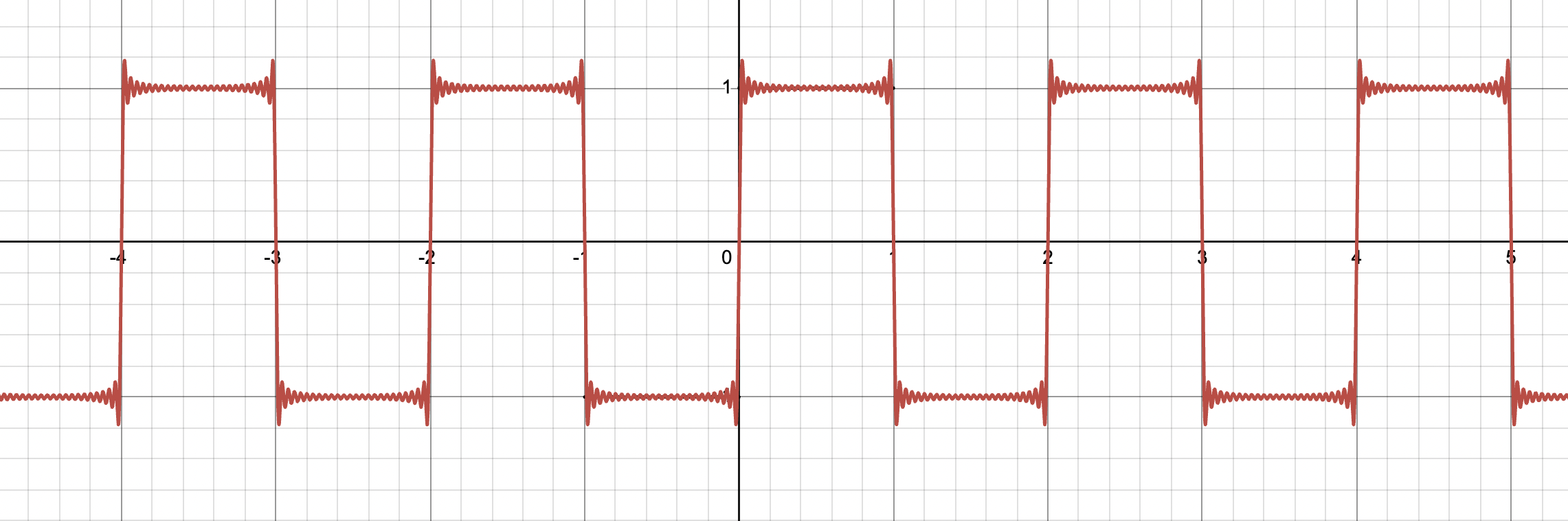
The partial sums \(S_N(x)\) of this series approximate \( f(x) \). Note that as \(x\) approaches a discontinuity of \( f(x) \) from either side, the value of \(S_N(x)\) tends to overshoot the limiting value of \( f(x) \)— either 1 or −1 in this case. This behavior of a Fourier series near a point of discontinuity of its function is typical and is known as Gibbs phenomenon.
3. Convergence Theorem
If \( f(x) \) is periodic and piecewise smooth, its Fourier series converges to:
-
\( f(x) \) at points where \( f \) is continuous.
- and at a point of discontinuity \( x_0\):
\[ \frac{f(x_0^+) + f(x_0^-)}{2}. \]
Example
Let \(f(t)\) be the \(2\pi\)-periodic function defined over one period by
Let \(\mathcal{F}(t)\) denote the Fourier series of \(f(t)\). Compute
Solution:
We use the Fourier series convergence theorem.
Step 1: Evaluate at \(t=0\)
\(f\) is continuous at \(0\):
Step 2: Evaluate at \(t=\pi\)
\(f\) is discontinuous at \(\pi\) (jump):
Step 3: Sum the values
Answer:
4. Use Fourier Series to Show Identities
Example
Let \( f(x) = |x| \) defined on \( (-\pi, \pi) \) and extended periodically with period \( 2\pi \). Use its Fourier series to compute the sum:
\[ \sum_{n=1,3,5,\dots}^{\infty} \frac{1}{n^2}. \]
Step 1: Recognize function type
\(f(x) = |x|\) is even, so its Fourier series contains only cosines:
Step 2: Compute \(a_0\)
Step 3: Compute \(a_n\)
Use symmetry: \(|x|\) is even, so double the integral from 0 to \(\pi\):
Integration by parts:
Step 4: Simplify for odd \(n\)
For odd \(n\), \((-1)^n = -1\), so:
Step 5: Evaluate series at \(x = 0\)
Fourier series at \(x=0\):
Step 6: Solve for the sum
Answer: