MA 30300 Notes | Sturm–Liouville Problems

Goal: Understand Sturm–Liouville problems, eigenvalues, orthogonality, and eigenfunction expansions.

1. Sturm–Liouville Problems

Definition: A Sturm–Liouville problem is an endpoint value problem of the form

\[ \frac{d}{dx}\left(p(x)\frac{dy}{dx}\right) - q(x)y + \lambda r(x)y = 0, \quad a < x < b \]

together with boundary conditions

\[ \alpha_1 y(a) - \alpha_2 y'(a) = 0, \quad \beta_1 y(b) + \beta_2 y'(b) = 0, \]

where neither \( \alpha_1, \alpha_2 \) both zero nor \( \beta_1, \beta_2 \) both zero. The parameter \( \lambda \) is the eigenvalue, whose allowable constant values are sought.

These problems are named after the French mathematicians Charles Sturm and Joseph Liouville, who investigated such problems in the 1830s.

Note that a Sturm–Liouville problem always has the trivial solution \( y(x) \equiv 0 \). We seek values of \( \lambda \), called eigenvalues, for which the problem admits a nontrivial real-valued solution \( y(x) \not\equiv 0 \). Such a solution is called an eigenfunction corresponding to \( \lambda \).

Example 1.1. We obtain different Sturm–Liouville problems by pairing the same differential equation

\[ y'' + \lambda y = 0, \quad 0 < x < L \]

with different homogeneous endpoint conditions:

\( y(0) = y(L) = 0 \)
\( y'(0) = y(L) = 0 \)
\( y(0) = y'(L) = 0 \)
\( y'(0) = y'(L) = 0 \)

2. Sturm–Liouville Eigenvalues

Theorem 1 (Sturm–Liouville Eigenvalues): Suppose the functions \( p(x), p'(x), q(x), r(x) \) are continuous on the interval \( [a,b] \), and that

\[ p(x) > 0, \quad r(x) > 0 \quad \text{for all } x \in [a,b]. \]

Then the eigenvalues of the Sturm–Liouville problem form an increasing sequence of real numbers

\[ \lambda_1 < \lambda_2 < \lambda_3 < \cdots < \lambda_n < \cdots \]

and satisfy

\[ \lim_{n \to \infty} \lambda_n = +\infty. \]

Furthermore, to within a constant multiple, there is exactly one eigenfunction \( y_n(x) \) associated with each eigenvalue \( \lambda_n \). In addition, if \( q(x) \ge 0 \) on \( [a,b] \) and the coefficients \(\alpha_1,\alpha_2,\beta_1,\beta_2\) are nonnegative, then all eigenvalues are nonnegative.

A Sturm–Liouville problem is called regular if it satisfies the hypotheses of Theorem 1, that is, it is regular if the following conditions hold:

The interval \([a,b]\) is finite (that is, \( -\infty < a < b < \infty \)).
The functions \( p(x), p'(x), q(x), r(x) \) are continuous on \( [a,b] \).
\( p(x) > 0 \) and \( r(x) > 0 \) on \( [a,b] \).

If any of these conditions fail, the Sturm–Liouville problem is classified as singular.

In this section we will confine our attention to regular Sturm–Liouville problems.

Example 2.1. Consider the Sturm–Liouville problem

\[ y'' + \lambda y = 0, \quad 0 < x < L, \] \[ y(0) = 0, \quad y(L) = 0. \]

Solving this problem leads to three cases \( \lambda < 0 \), \( \lambda = 0 \), and \( \lambda > 0 \). Only the positive case produces nontrivial solutions. The eigenvalues are

\[ \lambda_n = \frac{n^2 \pi^2}{L^2}, \quad n = 1,2,3,\dots \]

and the corresponding eigenfunctions are

\[ y_n(x) = \sin\left(\frac{n\pi x}{L}\right), \quad n = 1,2,3,\dots \]

Here we identify \( p(x) = 1 \), \( r(x) = 1 \), \( q(x) = 0 \), and boundary coefficients \( \alpha_1 = \beta_1 = 1 \), \( \alpha_2 = \beta_2 = 0 \). Thus, by Theorem 1, all eigenvalues are nonnegative.

Example 2.2. Find the eigenvalues and associated eigenfunctions of the Sturm–Liouville problem

\[ y'' + \lambda y = 0, \quad 0 < x < L, \] \[ y(0) = 0, \quad h y(L) + y'(L) = 0, \quad h > 0. \]

Solution: This problem satisfies the hypotheses of Theorem 1 with \( \alpha_1 = 1 \), \( \alpha_2 = 0 \), \( \beta_1 = h > 0 \), and \( \beta_2 = 1 \). Hence there are no negative eigenvalues.

First consider \( \lambda = 0 \). Then the differential equation becomes

\[ y'' = 0 \quad \Rightarrow \quad y(x) = Ax + B. \]

Applying \( y(0) = 0 \) gives \( B = 0 \), so \( y(x) = Ax \). Applying the second boundary condition:

\[ h y(L) + y'(L) = 0 \Rightarrow h(AL) + A = A(hL + 1) = 0. \]

Since \( h > 0 \), this forces \( A = 0 \), so only the trivial solution exists. Therefore, \( \lambda = 0 \) is not an eigenvalue.

For \( \lambda > 0 \), write \( \lambda = \mu^2 \). Then

\[ y(x) = A \cos(\mu x) + B \sin(\mu x). \]

Applying \( y(0) = 0 \) gives \( A = 0 \), so

\[ y(x) = B \sin(\mu x). \]

Applying the second boundary condition:

\[ h B \sin(\mu L) + B \mu \cos(\mu L) = 0. \]

For nontrivial solutions \( B \neq 0 \), we have

\[ h \sin(\mu L) + \mu \cos(\mu L) = 0, \]

Remark: If \( \cos(\mu L) = 0 \), then

\[ \mu L = \frac{\pi}{2} + n\pi, \quad n = 0,1,2,\dots \implies \sin(\mu L) = \pm 1 \]

Substituting into the boundary condition

\[ \pm h = 0 \]

which contradicts \( h > 0 \). Therefore,

\[ \cos(\mu L) \ne 0. \]

We divide by \( \cos(\mu L) \) (nonzero) to obtain

\[ \tan(\mu L) = -\frac{\mu}{h} = -\frac{\mu L}{h L}. \]

Let \( x = \mu L \). Then this becomes

\[ -\tan x = \frac{x}{hL}. \]

Graph showing the function y = -tan(x) in red with repeating vertical asymptotes at x = (2n-1)π/2, and the line y = x/(hL) in blue. The graphs intersect once in each interval between asymptotes, forming an infinite sequence of solutions that approach the asymptotes as n increases. — Intersections of \( y(x) = -\tan x \) and \( y(x) = x/(hL) \). Check out this desmos graph.

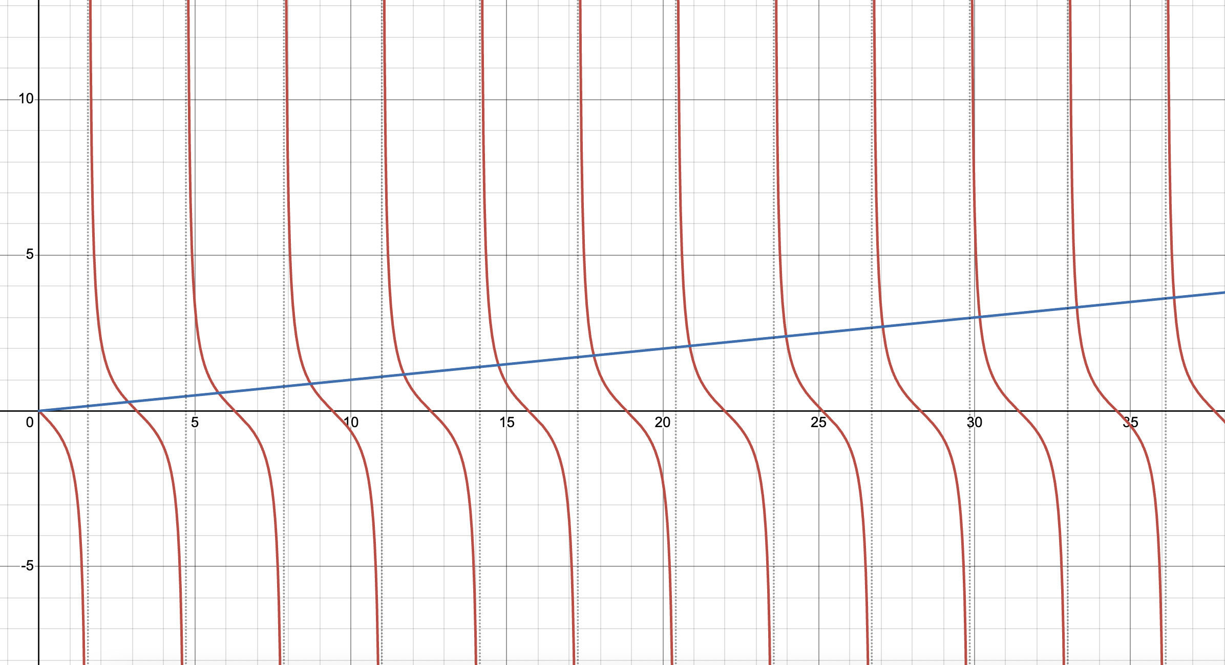
The solutions \( x = \mu L \) of this equation are the points of intersection of the graphs \( y(x) = -\tan x \) and \( y(x) = x/(hL) \). From the graph, there is an infinite sequence of positive roots

\[\mu_n L \in \{ \beta_1, \beta_2, \beta_3, \dots \} \]

and for large \( n \), \( \beta_n \) is close to \( \frac{(2n-1)\pi}{2} \). The eigenvalues and eigenfunctions are

\[ \lambda_n = \mu_n^2 = \frac{\beta_n^2}{L^2}, \qquad y_n(x) = \sin\left(\frac{\beta_n x}{L}\right), \quad n = 1,2,3,\dots \]

3. Orthogonal Eigenfunctions

Two functions \( \phi(x) \) and \( \psi(x) \) are said to be orthogonal on the interval \( [a,b] \) with respect to the weight function \( r(x) \) if

\[ \int_a^b \phi(x)\,\psi(x)\,r(x)\,dx = 0. \]

The following theorem shows that any two eigenfunctions of a regular Sturm–Liouville problem corresponding to distinct eigenvalues are orthogonal with respect to the weight function \( r(x) \).

Theorem 2 (Orthogonality of Eigenfunctions):

If the Sturm–Liouville problem is regular, then any two eigenfunctions corresponding to distinct eigenvalues are orthogonal with respect to the weight function \( r(x) \); that is,

\[ \int_a^b y_i(x)\,y_j(x)\,r(x)\,dx = 0, \quad \lambda_i \ne \lambda_j. \]

Example 3.1. Consider the Sturm–Liouville problem

\[ y'' + \lambda y = 0, \quad 0 < x < \pi, \] \[ y(0) = 0, \quad y(\pi) = 0. \]

Eigenvalues and Eigenfunctions:

The eigenvalues are

\[ \lambda_n = n^2, \quad n=1,2,3,\dots \]

The corresponding eigenfunctions are

\[ y_n(x) = \sin(nx). \]

Orthogonality:

These eigenfunctions are orthogonal on \( [0,\pi] \), since

\[ \int_0^\pi \sin(nx)\,\sin(mx)\,dx = 0, \quad n \ne m. \]

4. Eigenfunction Expansions

Theorem 3 (Eigenfunction Expansion / Completeness):

Let \( \{y_n(x)\} \) be the eigenfunctions of a regular Sturm–Liouville problem. Then any piecewise smooth function \( f(x) \) on \( [a,b] \) can be represented as a generalized Fourier series:

\[ f(x) \sim \sum_{n=1}^{\infty} c_n \, y_n(x). \]

The coefficients are given by

\[ c_n = \frac{\int_a^b f(x)\,y_n(x)\,r(x)\,dx}{\int_a^b y_n^2(x)\,r(x)\,dx}. \]

To determine the coefficients \( c_1, c_2, c_3, \dots \), we generalize the technique used to find ordinary Fourier coefficients in Section 9.1. First, we multiply both sides of the expansion by \( y_m(x)\,r(x) \) and integrate over the interval \( [a,b] \):

\[ \int_a^b f(x)\,y_m(x)\,r(x)\,dx = \int_a^b \left( \sum_{n=1}^{\infty} c_n y_n(x) \right) y_m(x)\,r(x)\,dx. \]

Using the orthogonality of the eigenfunctions, all terms vanish except when \( n = m \), which allows us to isolate \( c_m \).

Example 4.1. Represent the function \( f(x) = 9x \) as a series of eigenfunctions of the Sturm–Liouville problem

\[ y'' + \lambda y = 0,\quad 0 < x < 1, \] \[ y(0)=0,\qquad h y(1) + y'(1)=0,\quad (h>0). \]

The eigenvalues and eigenfunctions are given by

\[ \lambda_n = \alpha_n^2 \] \[ y_n(x) = \sin(\alpha_n x). \]

where \(\alpha_n\) are positive solutions of

\[ \tan x = -\frac{x}{h} \]

\[ y_n(x) = \sin(\alpha_n x). \]

Solution:

We expand \( f(x) = 9x \) in terms of the eigenfunctions:

\[ 9x = \sum_{n=1}^{\infty} c_n \sin(\alpha_n x), \]

where

\[ c_n = \frac{\int_0^1 9x \sin(\alpha_n x)\,dx} {\int_0^1 \sin^2(\alpha_n x)\,dx}. \]

First compute the numerator:

\[ \begin{aligned} I_n &= \int_0^1 9x \sin(\alpha_n x)\,dx \end{aligned} \]

Use integration by parts:

\[ \begin{aligned} u &= 9x \quad &dv &= \sin(\alpha_n x)\,dx \\ du &= 9\,dx \quad &v &= -\frac{\cos(\alpha_n x)}{\alpha_n} \end{aligned} \]

Apply the formula \( \int u\,dv = uv - \int v\,du \):

\[ \begin{aligned} I_n &= \left[ -\frac{9x\cos(\alpha_n x)}{\alpha_n} \right]_0^1 + \int_0^1 \frac{9\cos(\alpha_n x)}{\alpha_n}\,dx \end{aligned} \]

Evaluate the boundary term:

\[ \begin{aligned} \left[ -\frac{9x\cos(\alpha_n x)}{\alpha_n} \right]_0^1 &= -\frac{9\cos(\alpha_n)}{\alpha_n} \end{aligned} \]

Compute the remaining integral:

\[ \begin{aligned} \int_0^1 \cos(\alpha_n x)\,dx &= \left[ \frac{\sin(\alpha_n x)}{\alpha_n} \right]_0^1 \\ &= \frac{\sin(\alpha_n)}{\alpha_n} \end{aligned} \]

Substitute back:

\[ \begin{aligned} I_n &= -\frac{9\cos(\alpha_n)}{\alpha_n} + \frac{9}{\alpha_n} \cdot \frac{\sin(\alpha_n)}{\alpha_n} \end{aligned} \]

Simplify:

\[ \begin{aligned} I_n &= \frac{9}{\alpha_n^2} \left(\sin(\alpha_n) - \alpha_n \cos(\alpha_n)\right) \end{aligned} \]

We have

\[ \int_0^1 9x \sin(\alpha_n x)\,dx = \frac{9}{\alpha_n^2} \left(\sin(\alpha_n)-\alpha_n \cos(\alpha_n)\right). \]

Using the boundary condition

\[ \tan(\alpha_n) = -\frac{\alpha_n}{h} \]

we obtain

\[ \alpha_n\cos(\alpha_n)=-h\sin(\alpha_n). \]

Hence the numerator becomes

\[ \begin{aligned} \int_0^1 9x \sin(\alpha_n x)\,dx &= \frac{9}{\alpha_n^2}\left(\sin(\alpha_n)-\alpha_n\cos(\alpha_n)\right) \\[6pt] &= \frac{9}{\alpha_n^2}\left(\sin(\alpha_n)+h\sin(\alpha_n)\right) \\[6pt] &= \frac{9(1+h)}{\alpha_n^2}\sin(\alpha_n) \end{aligned} \]

Next compute the denominator:

\[ \begin{aligned} J_n &= \int_0^1 \sin^2(\alpha_n x)\,dx \\[6pt] \sin^2(\alpha_n x) &= \frac{1-\cos(2\alpha_n x)}{2} \\[6pt] J_n &= \int_0^1 \frac{1-\cos(2\alpha_n x)}{2}\,dx \\[6pt] &= \frac{1}{2}\int_0^1 1\,dx - \frac{1}{2}\int_0^1 \cos(2\alpha_n x)\,dx \\[6pt] &= \frac{1}{2}\Big[x\Big]_0^1 - \frac{1}{2}\Big[\frac{\sin(2\alpha_n x)}{2\alpha_n}\Big]_0^1 \\[6pt] &= \frac{1}{2} - \frac{1}{2}\cdot \frac{\sin(2\alpha_n)}{2\alpha_n} \\[6pt] &= \frac{1}{2}-\frac{\sin(2\alpha_n)}{4\alpha_n} \end{aligned} \]

\[ \int_0^1 \sin^2(\alpha_n x)\,dx = \frac{1}{2}-\frac{\sin(2\alpha_n)}{4\alpha_n}. \]

Therefore,

\[ \begin{aligned} c_n &= \frac{\frac{9(1+h)}{\alpha_n^2}\sin(\alpha_n)} {\frac{1}{2}-\frac{\sin(2\alpha_n)}{4\alpha_n}} \\[10pt] &= \frac{9(1+h)\sin(\alpha_n)}{\alpha_n^2} \cdot \frac{1}{\frac{1}{2}-\frac{\sin(2\alpha_n)}{4\alpha_n}} \\[10pt] &= \frac{9(1+h)\sin(\alpha_n)}{\alpha_n^2} \cdot \frac{4\alpha_n}{2\alpha_n-\sin(2\alpha_n)} \\[10pt] &= \frac{36(1+h)\alpha_n \sin(\alpha_n)} {\alpha_n \left(2\alpha_n-\sin(2\alpha_n)\right)} \end{aligned} \]

Final answer:

\[ c_n = \frac{36(1+h)\sin(\alpha_n)} {\alpha_n\left(2\alpha_n-\sin(2\alpha_n)\right)}. \]

5. Other examples

Example 5.1: Find the eigenvalue/eigenfunction pair corresponding to the smallest eigenvalue for the Sturm–Liouville problem

\[ y'' + \lambda y = 0,\quad 0 < x < 3\pi, \] \[ y(0)=0, \] \[ y(3\pi) - y'(3\pi)=0. \]

\( y_0=\sinh(kx) \) and \( \lambda_0=-k^2 \) where \( k \) is the smallest solution to \( \tanh(3\pi k)=k \) (Correct)
\( y_0=\cosh(kx) \) and \( \lambda_0=-k^2 \) where \( k \) is the smallest solution to \( \tanh(3\pi k)=k \)
\( y_0=1 \) and \( \lambda_0=0 \)
\( y_0=\sin(kx) \) and \( \lambda_0=k^2 \) where \( k \) is the smallest solution to \( \tan(3\pi k)=k \)
\( y_0=\cos(kx) \) and \( \lambda_0=k^2 \) where \( k \) is the smallest solution to \( \tan(3\pi k)=k \)

Solution:

For the smallest eigenvalue, set \( \lambda = -k^2 \), \( k>0 \). Then

\[ y'' - k^2 y = 0. \]

The general solution is

\[ y(x) = A\sinh(kx) + B\cosh(kx). \]

Apply \( y(0)=0 \):

\[ B=0 \quad \Rightarrow \quad y(x)=A\sinh(kx). \]

Apply \( y(3\pi)-y'(3\pi)=0 \):

\[ A\sinh(3\pi k) - Ak\cosh(3\pi k)=0. \]

Hence

\[ \tanh(3\pi k)=k. \]

Since the equation \( \tanh(3\pi k)=k \) has exactly one positive solution, denote it by \( k_0 \). Hence the eigenvalue is

\[ \lambda_0 = -k_0^2 \]

The eigenfunction is

\[ y_0(x)=\sinh(k_0 x) \]

Final eigenpair:

\[ (\lambda_0, y_0) = \left(-k_0^2,\; \sinh(k_0 x)\right), \quad \text{where } \tanh(3\pi k_0)=k_0. \]

Example 5.2:

The Sturm–Liouville problem

\[ \begin{array}{l} y''+\lambda y=0,\quad 0 < x < 1 \\ y(0)=0 \\ y(1)+y'(1)=0 \end{array} \]

has eigenvalues \( \lambda_n=\beta_n^2 \), where \( \beta_n \) are the positive solutions of \( \tan(\beta)=-\beta \), such that \( \beta_1 < \beta_2 < \cdots \), and eigenfunctions \( y_n=\sin(\beta_n x) \), which are mutually orthogonal. If the function \( f(x)=1 \) is expanded using these eigenfunctions,

\[ 1 \sim \sum_{n=1}^{\infty} c_n y_n = \sum_{n=1}^{\infty} c_n \sin(\beta_n x), \]

find \( c_n \).

Choose the correct answer:

\( c_n=\dfrac{4-4\cos(\beta_n)}{2\beta_n-\sin(2\beta_n)} \)
\( c_n=\dfrac{4-4\sin(\beta_n)}{2\beta_n-\cos(2\beta_n)} \)
\( c_n=\tan(4\beta_n) \)
\( c_n=\tan(2\beta_n) \)
\( c_n=\tan(\beta_n) \)

Solution:

We expand \( f(x)=1 \) in terms of the eigenfunctions:

\[ 1 \sim \sum_{n=1}^{\infty} c_n \sin(\beta_n x), \quad \text{where } \tan(\beta_n)=-\beta_n. \]

The coefficients are given by orthogonality:

\[ c_n = \frac{\int_0^1 \sin(\beta_n x)\,dx} {\int_0^1 \sin^2(\beta_n x)\,dx}. \]

Numerator:

\[ \begin{aligned} \int_0^1 \sin(\beta_n x)\,dx &= \left[-\frac{\cos(\beta_n x)}{\beta_n}\right]_0^1 \\[6pt] &= \frac{1-\cos(\beta_n)}{\beta_n} \end{aligned} \]

Denominator:

\[ \begin{aligned} I &= \int_0^1 \sin^2(\beta_n x)\,dx \\[6pt] &= \int_0^1 \frac{1-\cos(2\beta_n x)}{2}\,dx \\[6pt] &= \frac{1}{2}\int_0^1 1\,dx - \frac{1}{2}\int_0^1 \cos(2\beta_n x)\,dx \\[6pt] &= \frac{1}{2}[x]_0^1 - \frac{1}{2}\left[\frac{\sin(2\beta_n x)}{2\beta_n}\right]_0^1 \\[6pt] &= \frac{1}{2} - \frac{1}{2}\cdot \frac{\sin(2\beta_n)}{2\beta_n} \\[6pt] &= \frac{2\beta_n-\sin(2\beta_n)}{4\beta_n} \end{aligned} \]

Combine:

\[ \begin{aligned} c_n &= \frac{\frac{1-\cos(\beta_n)}{\beta_n}} {\frac{2\beta_n-\sin(2\beta_n)}{4\beta_n}} \\[10pt] &= \frac{1-\cos(\beta_n)}{\beta_n} \cdot \frac{4\beta_n}{2\beta_n-\sin(2\beta_n)} \\[10pt] &= \frac{4(1-\cos(\beta_n))}{2\beta_n-\sin(2\beta_n)} \end{aligned} \]

Final answer:

\[ c_n=\frac{4-4\cos(\beta_n)}{2\beta_n-\sin(2\beta_n)} \]

Correct answer: A